In this post, connected components of the world map graph are identified using the Correlates of War (COW) Direct Contiguity dataset v 3.2. This has data current as of end-2016. In line with the previous post, we define connected components to be sets of countries that are connected to each other by a land or river border.
The world map is different from the contiguous US map in that there are many countries or sets of countries that are disconnected from others. Thus it is not necessary that a certain country be reachable from any other country over land routes. Since the dataset only provides pairs of countries that share borders (i.e. the edges of our graph), the union of these countries will not cover all countries in the world. e.g. Australia does not share a land or river border with any country and thus will not appear in the list of edges. So a different data source is needed to get a list of all countries.
Some countries themselves contain territories physically disconnected by sea or ocean but they have been treated as a single entity e.g. in addition to the mainland, Malaysia has a some territory that is a portion of an island whose remainder belongs to Indonesia. Thus Malaysia is treated as being connected to Indonesia though one cannot reach any part of Indonesia from the Malaysian mainland via land. Similarly separate islands of a country are implicitly regarded as being connected.
Another twist is that the COW dataset uses its own country codes while standard map libraries work with ISO3 country codes. Converting from COW to ISO3 country codes is thus needed.
Based on these needs, an R script worldCountriesProcessor.R is used to generate a list of ISO3 codes for all countries and to convert the COW codes in the dataset to ISO3 codes. The main reason for using R for this transformation is the availability of a ready-made countrycode package that makes it easy to do conversions and also to list out all countries for a particular code system. The data used by this package is also available here and the conversion can be implemented in Python instead with just a little more work.
When trying to do conversion of country codes, a problem was faced in converting the COW code KOS which is for Kosovo. It turns out that Kosovo unilaterally declared independence from Serbia in 2008 and an official ISO3 code is not defined for it. However, within EU, KSV is the 3-letter country code that is used for it. So in worldCountriesProcessor.R, KOS -> SRB conversion is incorporated as a special exception.
An alternative approach would have been to add KSV as a country. But the COW country codes do not include Serbia which is an ISO recognized country with ISO3 code SRB ! Issues like this are often encountered when handling datasets and call for more detailed study and reconciliation which is out of scope for this post and we simply use an easy solution of replacing KOS with SRB.
The R script uses the contdir.csv file as its input and generates two files in the data directory :-
i) all-countries-iso3.dat - a list of 3-letter iso3 codes for all countries in the world
ii) country-borders-landorriver-iso3.dat - pairs of countries (iso3 codes) that share a land or river border in end-2016 as per the CoW Contiguity dataset (=> conttype==1, end==201612)
In terms of graphs, i) is the set of vertices and ii) is the set of undirected edges.
The countrycode package installation and the execution of the R script to generate the above files is shown below.
> R --vanilla
> install.packages('countrycode',repos='http://cran.us.r-project.org')
...
> Rscript worldCountriesProcessor.R
 Number of countries/nodes (N) = 256
 Generated output data file containing list of all countries (ISO3) : data/all-countries-iso3.dat
 Number of countries with land or river border(s) (Nbar) = 158 ; Number of borders/edges M = 316
 Generated output data file containing neighbor country pairs (ISO3) : data/country-borders-landorriver-iso3.dat
The messages say that there are 256 countries in all-countries-iso3.dat and 316 edges defined in country-borders-landorriver-iso3.dat. 158 countries out of the 256 appear in the list of edges.
Once the graph data is ready, the Python script from the previous post i.e. graphProcessor.py can be executed and it generates the connected component ids for each country in an output file. The graph algorithm used to calculate the connected components is based on the standard one - start a DFS from every unvisited vertex and mark all vertices visited by a particular DFS invocation with the same connected component id. Refer to the entry point method dfs_main_disconnected in the Python script for details.
A separate html file contains Javascript code that utilizes the D3 DataMap library to display and label the connected components which show up on mouse hover. A static screenshot is provided below.
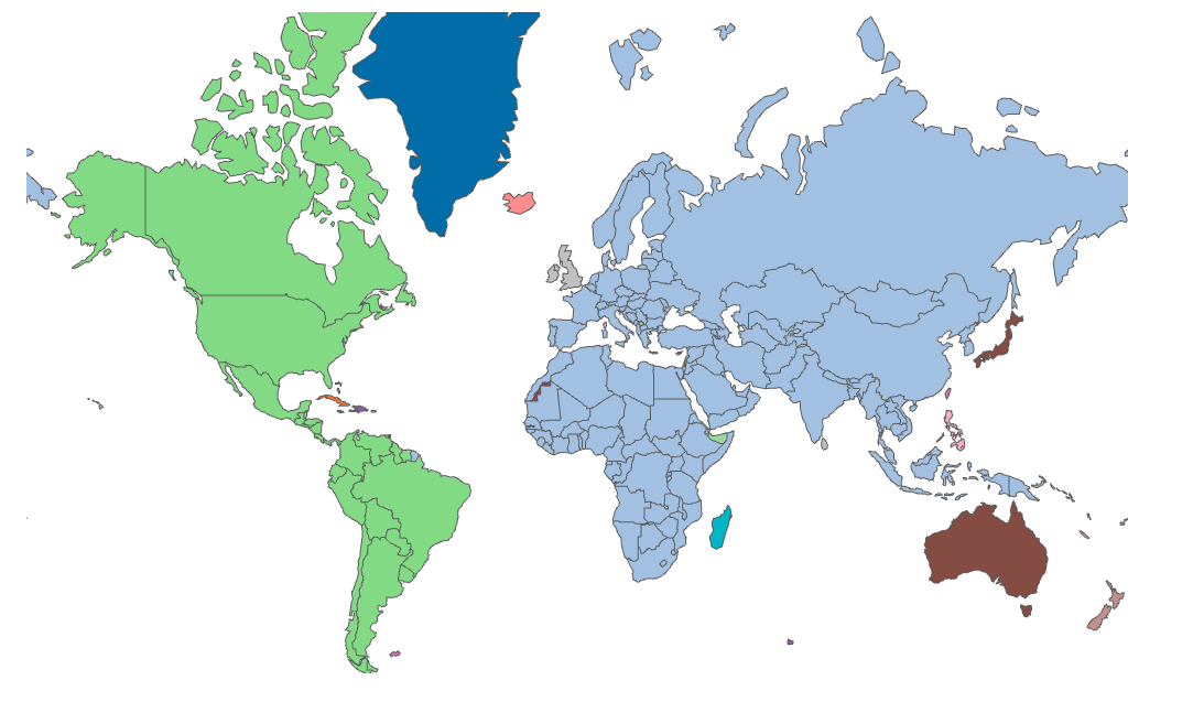
The interactive view is available here. It may take a few seconds for the map to be rendered the first time.
A couple of potential problems surface directly and these have to do with French Guiana and Western Sahara shown below.
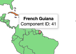
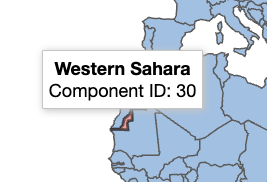
These show up as disconnected from the big surrounding connected component that they should be part of. The explanations are found quite easily. Western Sahara is a disputed territory and French Guiana is regarded as part of France and the EU. Thus, both have special characteristics associated with them that affect the definition of borders.