Code
theta = range(1,101)
fig = plt.figure(figsize=(7,7))
r = theta

plt.polar(r, theta, 'bo')
plt.show()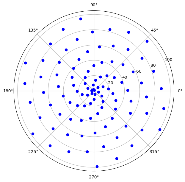
Recently I came across an amazing 3blue1brown video titled Why do prime numbers make these spirals ? It covers Archimedian spirals generated using polar co-ordinates (also covered in one of my prior posts Generating Spirals). Then it moves on to rational approximations for \(\pi\), modular arithmetic, residue classes modulo prime numbers, coprimes, the Euler Totient function and finally Dirichlet’s theorem that deals with the distribution of primes. All in all, a heady mix indeed !
There is also an accompanying detailed writeup from 3blue1brown available here. There are a number of important areas touched upon by the video and it was very stimulating to watch it a number of times. Intrigued by it, I did some of my own experimentation on the visualization of these spirals and have compiled some of my learnings and observations below.
In an earlier post Generating Spirals, we had seen that Archimedian spirals are described by the polar equation \(\ r = a\theta\) where ‘a’ is a constant. In the 3blue1brown video, the discussion centers around a particular subset of such spirals, viz. where a=1. Thus, the polar equation is \(r = \theta\)
Further, only points where \(\theta\), and thus \(r\), have integer values are considered. The core theme is the visual patterns that arise by plotting just these points.
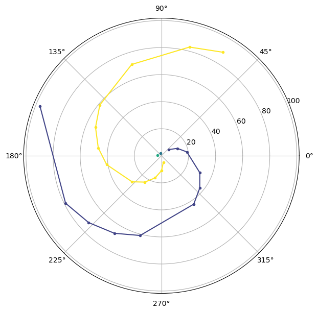
We plot the first 100 points which are basically the set of polar co-ordinates \((\theta, \theta)\) where \(\theta\) takes integer values in the range [1,100].
theta = range(1,101)
fig = plt.figure(figsize=(7,7))
r = theta
plt.polar(r, theta, 'bo')
plt.show()
There are 6 spiral arms that clearly show up in the plot above. But we plotted 100 points (with polar co-ordinates (n,n) where n is a positive integer) for a single Archimedian spiral only !
Let’s delve more into what is going on !
We join the dots with straight line segments (straight for simplicity !) and it becomes certain that all the points indeed lie on a single Archimedian spiral i.e. the one with polar equation \(r = \theta\)
Notice that the corresponding vertices of the unfolding “hexagons” below seem to be on the six apparent spirals. So the spiral arms are only something we are perceiving. Our eyes are seeing them emerge !
r = range(0,51)

fig = plt.figure(figsize=(7,7))
plt.polar(r, r, 'bo--')
plt.show()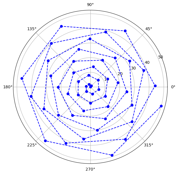
Let us now show each spiral of the 6 spiral arms in a different colour to make things clearer. This matches the type of visualization that is used in the video. Basically we can associate the points associated with integers that are a step size 6 apart.
For example, the first spiral arm has points (0,0), (6,6), (12,12) … and is marked in brown.
The second spiral arm is composed of (1,1), (7,7), (13,13) … and the third has (2,2), (8,8), (14,14)… The sixth and last spiral arm is made up of (5,5), (11,11), (17,17)… and is marked in yellow. Note that if we start with (6,6), we will repeat the first spiral. If we start with (7,7), we will repeat the second and so on. Thus, we can hae only six spiral arms and no more.
In other words, the six spiral arms correspond to the six residue classes mod 6 on the set of non-negative integers. This is because six remainders or residues, i.e. 0,1,2,3,4,5, can arise when non-negative integers are divided by 6.
%matplotlib inline

def plot_points(user_choice, filter_primes=False, size=(10,10)):
    fig, ax = plt.subplots(figsize=size, subplot_kw={'projection': 'polar'})

    match(user_choice):
        case 1:
            # Case 1: 6 ~ 2*pi, plot 100 points
            stop, step = 100,6

        case 2:
            # Case 2: 44 ~ 7*2π  π ~ 22/7
            stop, step = 1000,44

        case 3:
            # Case 3: 710 ~ 113*2π *  π ~ 335/113
            stop,step= 10000,710

        case 4:
            stop, step = 100, 8
        case _:
            print("Provide numeric value 1,2, 3 or 4 only. [${user_choice}] is not a valid input")
            return -1

    # Use a colormap to generate a list of colors
    colormap = plt.cm.viridis
    colors = colormap(np.linspace(0, 1, num=step)) # Refer https://matplotlib.org/3.1.1/tutorials/colors/colormap-manipulation.html


    pt_vals = range(0,step)

    for i in pt_vals:
        r = np.arange(start=i,stop=stop,step=step,dtype=int)
        if(filter_primes):
            r = list(filter(is_prime, r))
        theta=r

        # Add a label only for the case with a small number of plots
        label = f'i = {i}' if user_choice == 1 else None

        ax.plot(r,theta,'.-',color=colors[i], label=label)

    if(filter_primes == True):
        return 1

    # Add a legend to the plot
    if(user_choice == 1):
        ax.legend(title=f"Residue class mod {step}", bbox_to_anchor=(1.1, 1.05))
    else:
        # Create a normalizer to map the values of 'i' to the colormap range [0, 1]
        norm = Normalize(vmin=1, vmax=step)
        # Create a ScalarMappable object that can be used to create the colorbar
        sm = ScalarMappable(cmap=colormap, norm=norm)
        # Add the colorbar to the figure
        cbar = fig.colorbar(sm, ax=ax, pad=0.1, shrink=0.8)
        cbar.set_label(f'Residue class mod {step}', rotation=270, labelpad=15)

    plt.show()
    return 0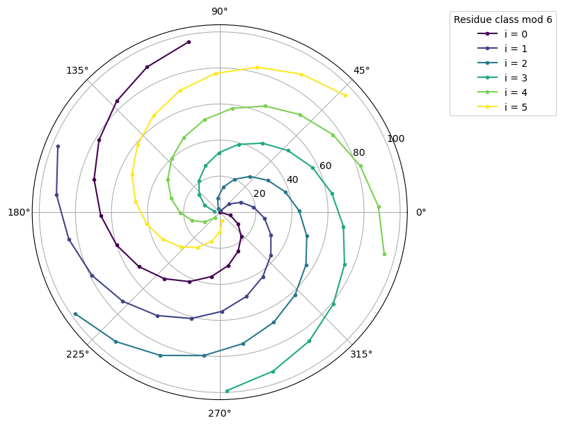
The above discussion generates a very important insight about the video.
Everything shown in the 3blue1brown video - all the various spiral patterns - are produced by points on a single Archimedian spiral !
All the different patterns of spiral arms are seen or perceived by us when different sets of points on that one spiral are selectively displayed.
Each spiral arm maps to a particular residue class of the step size or modulus involved.
So far, we have looked at only one step size or modulus i.e. 6. We will look at some others in the next section and that will take us into rational approximations for \(\pi\) !
We move on the area of rational approximations to \(\pi\) that the video leads us into later through the spirals. Note that this is not about the “prime spirals” alone. Although the video starts off with “prime” spirals, they point out later that spiral arms and the prime filtering are orthogonal aspects.
Now we will look at two important concepts that come out on further exploration on the ideas illustrated in the video :- 1. Only a few specific step sizes or moduli produce spiral arms e.g. 6, 44, 710. Others do not ! 2. When we consider 6, 44 and 710, the spiral arms become straighter i.e. they approach straight lines.
With regard to point 1, the plot below shows what happens when a step size of 8 is used ! It is quite a mess and we see jagged patterns that go all over the place. So why is it the case ?
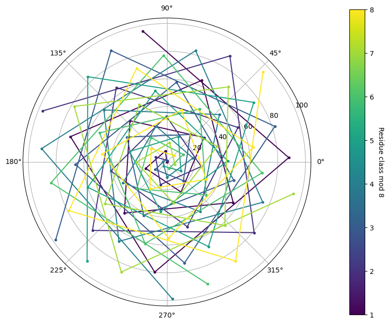
This leads us into point 2. Only those step sizes or moduli that are close enough to \(2\pi\) produce spiral arms. And this is because, a rotation by something close to \(2\pi\) puts the next point close to the radial line passing through the origin and the current point. This is what produces the spirals.
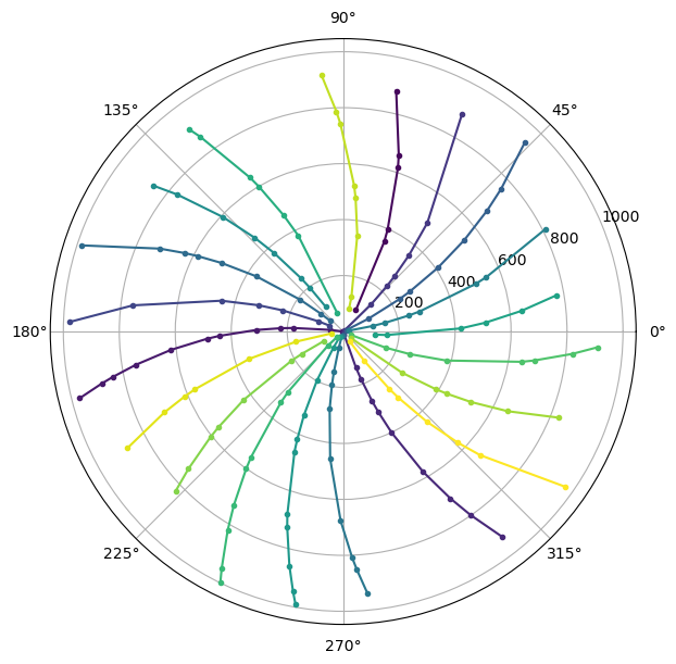
Next we show what happens with step sizes or moduli of 44 and 710.
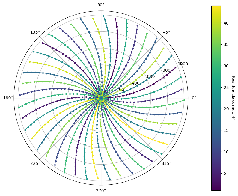
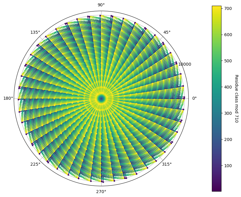
The spiral arms have become gentler or less curved with a modulus of 44. And when the modulus is 710, the spiral arms have effectively become straight lines !
The reason for this lies in the fact that 44 is a closer approximation to an integer multiple of 2\(\pi\) than 6 is. And 710 is even closer to an integer multiple of \(2\pi\).
If we rotate a radial line by a multiple of \(2\pi\), it comes back to its original position. Thus the successive points lie on the same radial line when the next point’s angular coordinate \(\theta\) is an increment of an integer multiple of \(2\pi\).
When these observations are summarized in a table, we can see the familar \(22/7\) rational approximation for \(\pi\) and also the less familar but more accurate \(355/113\).
| S.No. | M (mod/step) | M/\(2\pi\) | n (Multiple No.) | Approx. \(\pi\) (rational) |
|---|---|---|---|---|
| 1 | 6 | 0.95493 | 1 | \(3\) |
| 2 | 44 | 7.00282 | 7 | \(22/7\) |
| 3 | 710 | 113.00001 | 113 | \(355/113\) |
This is one of the important areas of the 3blue1brown video and actually the trigger for the creation of it. Refer this Math Stack Exchange post. They talk about the distribution of primes and Dirichlet’s theorem as part of the exploration. However, a more important point they make is that the spiral arms and prime numbers have only an incidental relationship.
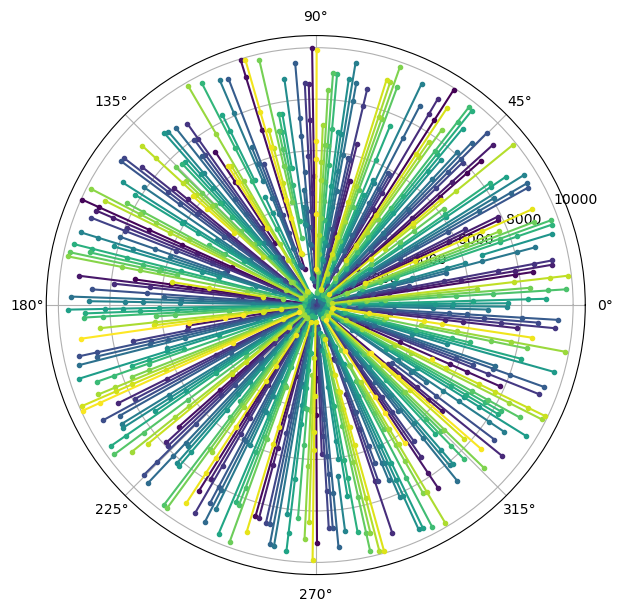
Just for completeness, we include the plots below when only prime number polar coordinates (p,p) are displayed with the same moduli i.e. 6, 44 and 710.
And with that we conclude this post.